Introduction
In this Excel lesson we will explain how to use Excel's VLOOKUP function. In addition, we will show an example of how to apply VLOOKUP to a fictional dataset.
VLOOKUP
When using Excel's VLOOKUP function we find that it has 3 required arguments and 1 optional argument. In particular, we have
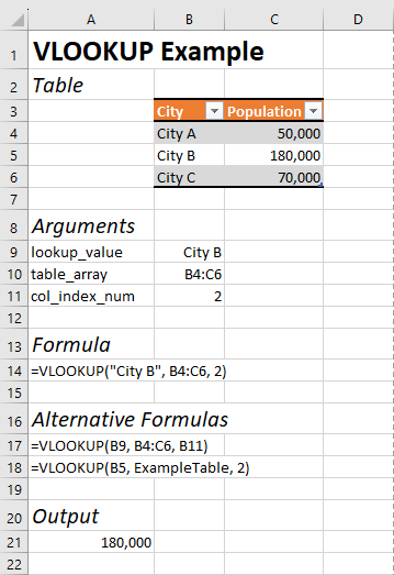
VLOOKUP(lookup_value, table_array, col_index_num, [range_lookup])
The idea is to match the lookup_value with a value in the cells table_array and return the corresponding value with column number col_index_num. Let's look at an example.
In this example, our table_array is the table ExampleTable. Due to limitations with VLOOKUP the first column in our table_array must include our lookup_value which in this example is City B. The goal of VLOOKUP is to match the first row in table_array that matches with our lookup_value and return the result in the specified column. In our case we set col_index_num as 2 and get the result 180,000.
WARNING: In this example we did not specify the optional range_lookup argument. This argument defaults to TRUE which means the result could be based on an approximate of our lookup_value. If you need an exact match this value should be set to FALSE.
To demonstrate that we can define our arguments in more than one way we include some alternate formulas in our example. So for example we can reference a string value by the cell it is in or surround it with quotation marks for our lookup_value. We can also reference a table by the table name or the absolute cells.
Application
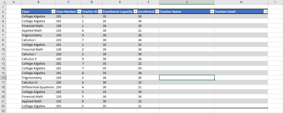
In our VLOOKUP application we have a sample of classes which students can enroll in. We will demonstrate how to apply VLOOKUP to get additional data from another table. Here is our table before applying VLOOKUP
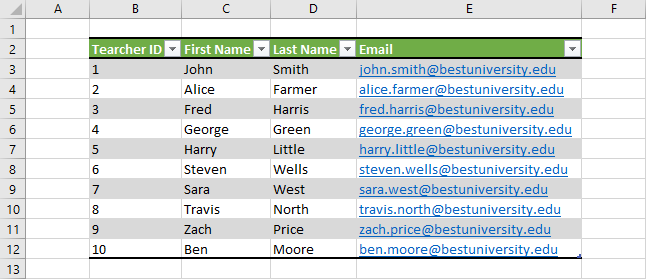
Notice that we currently do not have any information about the teachers' names or email addresses. All we have is a Teacher ID. What we do have is a table called Teachers with this information. Our goal is to use VLOOKUP to bring this data into our Classes table.
Let's consider how to get the teachers' email addresses into our Classes table first. We extract a teacher's email address using the following formula for each row in the Teacher Email column:
=VLOOKUP([@[Teacher ID]], Teachers, 4, FALSE)
Thus our lookup_value is the Teacher ID, our table_array is the Teachers table, our col_index_num is 4, and our range_lookup is FALSE.`
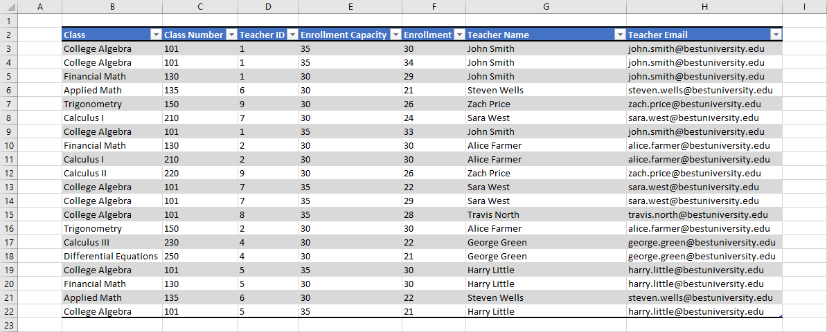
To fill the Teacher Name column we do something similar, but utilize the CONCATENATE function to combine our first and last names together. Our required formula for the Teacher Name column is:
=CONCATENATE(VLOOKUP([@[Teacher ID]],Teachers,2,FALSE)," ",VLOOKUP([@[Teacher ID]],Teachers,3,FALSE))
Putting everything together we get our complete Classes table.
WARNING: Since we reference a table by its column number, if we add a new column to the reference table before the referenced column our results will be wrong. This will require a manual update of the VLOOKUP formula to fix this issue.
Conclusion
VLOOKUP is a powerful way to get information from one table to another. In fact, we saw in our example that VLOOKUP can be used in a similar manner to a LEFT JOIN in SQL. The biggest drawback of VLOOKUP, however, is how ridged it can be. For example, it does not know how to respond to an insertion of a new column into the table_array that occurs before the referenced col_index_num.
Overall, it is pretty useful that we can get SQL like functionality with Excel through the use of VLOOKUP.
Add a new comment